Observadores de estado
Cuándo no se conoce o no se puede medir una variable de estado para en el sistema a controlar, se deben emplear métodos para calcular dichas señales.
Para obtener un valor aproximado del vector de estado se utiliza una estructura denominada Observador.
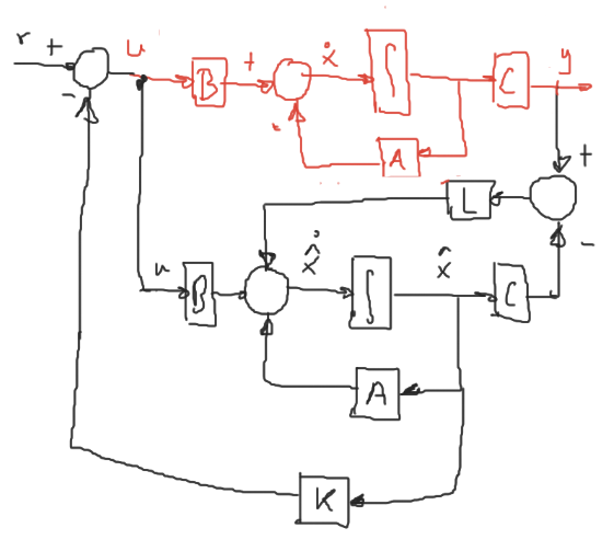
La retroalimentación de estado $u = r - kx$ asume que se tienen disponibles todas las variables de estado. Sin embargo si no se puede se aplica la siguiente estructura:
Haciendo $u=r - k\hat{x}$. Donde $\hat{x}$ es un valor aproximado de $x$.
Los observadores de estado pueden ser de orden completo o orden reducido. La diferencia es que el de orden reducido sólo reproduce las señales no conocidas y las de orden completo todas las señales, incluso las ya conocidas. Sin embargo, la estructura del de orden completo es más sencilla.
Considere el sistema SISO
Donde la entrada $u$ y la salida $y$, son conocidas.
Se asume que el vector de estado $x$ es parcial o totalmente desconocido.
El problema consiste en estimar $x$ a partir de $u$ y de $y$.
Estructura Luenberger
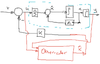
El observador de estado para el sistema (1) se define como sigue:
\[(2)\ \dot{\hat{x}} = \underbrace{A\hat{x} + Bu}_\text{copia del sistema} + \underbrace{L(y-C\hat{x})}_\text{Factor de correción}\quad,\quad \hat{x}(0) = x_0\]Donde $L:n\times 1$ porque es un sistema con una salida.
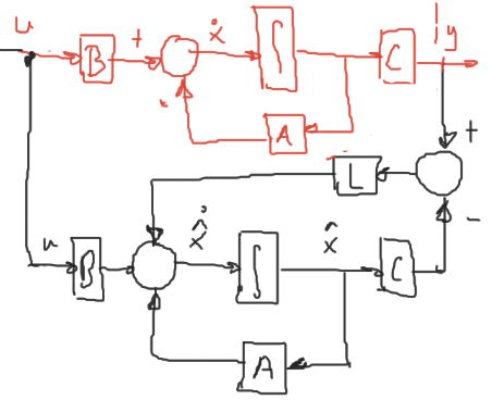
En rojo, aparece el sistema original, en negro el observador de estado.
Al aplicar retroalimentación sería de la siguiente forma:
Reescribiendo (2)
\[\begin{aligned} \dot{\hat{x}} &= A\hat{x} + Bu + L(y-C\hat{x})\\ &= (A-LC)\hat{x} + Bu + Ly\\ &= (A-LC)\hat{x} + [B\ L]\underbrace{\begin{bmatrix}u\\y\end{bmatrix}}_\text{Entradas}\\ \end{aligned}\]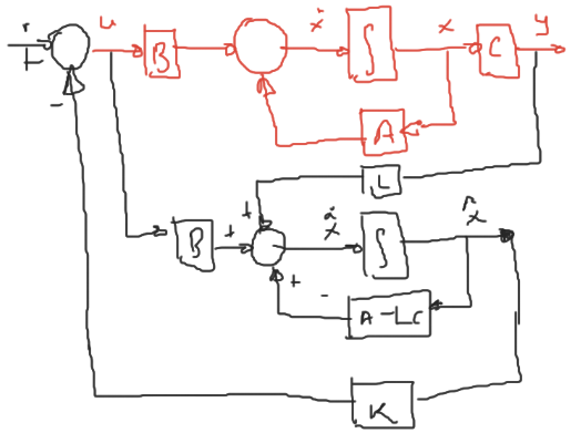
Se define el error de estimación como,
\[(3)\quad e = x - \hat{x}\]Derivando (3)
\[(4)\quad \dot{e} = \dot{x} - \dot{\hat{x}}\]Sustituyendo (1) y (2) en (4),
\[\begin{aligned} \dot{e} &= Ax + Bu - A\hat{x} - Bu - L(y-C\hat{x})\\ &= Ax - A\hat{x} - Ly + LC\hat{x}\\ &= Ax - A\hat{x} - LCx + LC\hat{x}\\ &= A(x - \hat{x}) - LC(x - \hat{x})\\ &= Ae - LCe\\ &= (A - LC)e\\ \end{aligned}\]Resolviendo la ecuación diferencial:
\[\boxed{e(t) = e^{(A-LC)t}e(0)}\] \[||e||\xrightarrow[t\rightarrow\infty]{} 0\quad \text{si}\quad \boxed{A-LC}\quad \text{es estable}\]Entonces el diseño del observador de estado se resuelve como un problema de ubicación de polos para la matriz $\boxed{A-LC}$, es decir, se debe calcular $L$ para asignar la dinámica deseada del observador.
Nota: El observador debe ser siempre más rápido que el controlador de otra forma el controlador actuaría sobre un sistema retrasado.
Ejercicio
Calcular la ganancia $L$ para asignar los polos del observador en $-2$, $-2\pm 2j$
\[\dot{x} = \begin{bmatrix} -1 & 1 & -2\\ 0 & -1 & 1\\ 0 & 0 & -1\\ \end{bmatrix}x + \begin{bmatrix} 1\\0\\1 \end{bmatrix}u\] \[y = [1\ 0\ 0]u\]clc; close all; clear all;
A = [-1 1 -2
0 -1 1
0 0 -1];
B = [1 0 1]';
C = [1 0 0];
syms s L1 L2 L3;
plcd = collect((s+2)*(s+2-2i)*(s+2+2i))
L = [L1;L2;L3];
I = eye(3);
plc = collect(det(s*I - (A - L*C)))
eq1 = L1 + 3 == 6;
eq2 = 2*L1 + L2 - 2*L3 + 3 == 16;
eq3 = L1 + L2 - L3 + 1 == 16;
L = solve([eq1 eq2 eq3],L1,L2,L3);
L = [L.L1;L.L2;L.L3]
eig(A-L*C)
Forma canónica controlable
\[\tilde{x} =\] \[x = S\tilde{x} = S\] \[\tilde{O} = O\]Considere el sistema SISO
El polinomio del sistema (1) es:
\[p(s) = \det(sI-A) = s^n + a_1 s^{n-1}+ a_2 s^{n-2} + \cdots + a_{n-1} s + a_n\]Si el sistema (1) es observable, entonces puede ser transformado en la forma canónica observable, haciendo
\[x = Sz\quad(2)\]Sustituyendo (2) en (1):
\[\begin{aligned} \dot{x} = S\dot{z} &= ASz + Bu\\ (3)\quad\dot{z} &= S^{-1}ASz + S^{-1}Bu = \mathcal{A}z + \mathcal{B}u\\ &= \begin{bmatrix} 0&0&0&\cdots&0&-a_{n}\\ 1&0&0&\cdots&0&-a_{n-1}\\ 0&1&0&\cdots&\vdots&\vdots\\ \vdots&\ddots&\ddots&\ddots&\ddots&-a_{2}\\ 0&\cdots&\cdots&0&1&-a_{1}\\ \end{bmatrix} \tilde{x} + \begin{bmatrix}bn\\ b_{n-1}\\ \vdots \\ b_2\\ b_1\end{bmatrix}u\\ \end{aligned}\] \[y = CSz = \begin{bmatrix}0&0&0&\cdots&1\end{bmatrix}z\]Donde,
\[\def\rddots{\cdot^{\normalsize\cdot^{\normalsize\cdot}}} S^{-1} = \tilde{O}^{-1}O = \begin{bmatrix} a_{n-1}&\cdots&a_3&a_2&a_1&1\\ \vdots&\rddots&\rddots&\rddots&1&0\\ a_3&\rddots&\rddots&\rddots&\rddots&\vdots\\ a_2&a_1&1&\rddots&&\vdots\\ a_1&1&0&&&\vdots\\ 1&0&\cdots&\cdots&\cdots&0\\ \end{bmatrix}\begin{bmatrix}C\\CA\\CA^2\\\vdots\\CA^{n-1}\end{bmatrix}\]El observador se propone para el sistema (3)
\[\dot{\hat{z}} = \underbrace{S^{-1}AS\hat{z} + S^{-1}Bu}_\text{copia del sistema} + \underbrace{\bar{L}(y-CS\hat{z})}_\text{Factor de correción}\quad,\quad \hat{z}(0) = z_0\] \[\begin{aligned} \dot{\hat{z}} &= S^{-1}AS\hat{z} + S^{-1}Bu + \bar{L}(y-CS\hat{z})\\ &= S^{-1}AS\hat{z} + S^{-1}Bu + \bar{L}y-\bar{L}CS\hat{z}\quad;\quad\bar{L} = S^{-1}L\\ &= S^{-1}AS\hat{z} + S^{-1}Bu + S^{-1}Ly-S^{-1}LCS\hat{z}\\ (5)\qquad &= S^{-1}(A-LC)S\hat{z} + S^{-1}Bu + \bar{L}y\\ \end{aligned}\] \[(6)\quad \begin{cases} \dot{\hat{x}} &= (A-LC)\hat{x} + Bu + Ly\\ y &= C\hat{x} \end{cases}\]Los observadores (5) y (6) son similares, es decir:
\[\lambda(S^{-1}(A-LC)S) = \lambda(A-LC)\]Por lo tanto:
\[\begin{aligned} \dot{\hat{z}} &= \mathcal{A}\dot{z} + \mathcal{B}u + \bar{L}(y-C\hat{z})\\ &= \mathcal{A}\dot{z} + \mathcal{B}u + \bar{L}y-\bar{L}C\hat{z}\\ &= (\mathcal{A}-\bar{L}C)\dot{z} + \mathcal{B}u + \bar{L}y\\ \end{aligned}\] \[\begin{aligned} p_{LC} &= det(sI-(A-LC)) = det(sI - P(A-LC)P^{-1})\\ &= s^n + \tilde{a}_1 s^{n-1}+ \tilde{a}_2 s^{n-2} + \cdots + \tilde{a}_{n-1} s + \tilde{a}_n\\ &= (s - \mu_1)(s - \mu_2)\cdots(s - \mu_n) \end{aligned}\]Donde $\mu_i$ son los polos del observador.
\[\begin{aligned} \mathcal{A} - \bar{L}C &= \begin{bmatrix} 0&0&0&\cdots&0&-\tilde{a}_{n}\\ 1&0&0&\cdots&0&-\tilde{a}_{n-1}\\ 0&1&0&\cdots&\vdots&\vdots\\ \vdots&\ddots&\ddots&\ddots&\ddots&-\tilde{a}_{2}\\ 0&\cdots&\cdots&0&1&-\tilde{a}_{1}\\ \end{bmatrix} = \begin{bmatrix} 0&0&0&\cdots&0&-a_{n}\\ 1&0&0&\cdots&0&-{a}_{n-1}\\ 0&1&0&\cdots&\vdots&\vdots\\ \vdots&\ddots&\ddots&\ddots&\ddots&-{a}_{2}\\ 0&\cdots&\cdots&0&1&-{a}_{1}\\ \end{bmatrix}\begin{bmatrix}\bar{L}_1\\\bar{L}_2\\\vdots\\\bar{L}_n\end{bmatrix}\begin{bmatrix}0&0&\cdots&0&1\end{bmatrix}\\ &= \begin{bmatrix} 0&0&\cdots&0&-a_n-\bar{L}_1\\ 1&0&\cdots&0&-a_{n-1}-\bar{L}_2\\ 0&1&\cdots&0&\vdots\\ 0&0&\cdots&1&-a_1-\bar{L}_n\\ \end{bmatrix} \end{aligned}\]Por lo tanto:
\[\begin{aligned} -\tilde{a}_n = -a_n - \bar{L}_1\quad&\Rightarrow\quad \bar{L_1} = \tilde{a_n} - a_n\\ -\tilde{a}_{n-1} = -a_{n-1} - \bar{L}_2\quad&\Rightarrow\quad \bar{L_2} = \tilde{a}_{n-1} - a_{n-1}\\ &\vdots\\ -\tilde{a}_{1} = -a_{1} - \bar{L}_n\quad&\Rightarrow\quad \bar{L_n} = \tilde{a}_{1} - a_{1}\\ \end{aligned}\]Entonces:
\[\bar{L} = \begin{bmatrix} \tilde{a}_n - a_n\\ \tilde{a}_{n-1} - a_{n-1}\\ \vdots\\ \tilde{a}_1 - a_1\\ \end{bmatrix}\]Procedimiento
- Determinar el polinomio característico del sistema (1), $p(s) =det(sI-A)$
\(a_1,a_2,\ldots,a_n\)
- Obtener el polinomio característico con los polos del observador
- Calcular $S^{-1}$ y luego $S$
- Calcular $\bar{L}$
- Obtener $L = S\bar{L}$
- Comprobación
eig(A-LC)
Fórmula de Ackerman
Considere el sistema SISO
El polinomio del sistema (1) es:
\[p(s) = \det(sI-A) = s^n + a_1 s^{n-1}+ a_2 s^{n-2} + \cdots + a_{n-1} s + a_n\]y el observador de estado:
\[(2)\quad \begin{cases} \dot{\hat{x}} &= A\hat{x} + Bu + L(y-C\hat{x})\\ \dot{\hat{x}} &= (A-LC)\hat{x} + Bu + Ly\\ \end{cases}\]El polinomio característico para el observador es:
\[\begin{aligned} p_{LC} &= det(sI-(A-LC)) = det(sI - P(A-LC)P^{-1})\\ &= s^n + \tilde{a}_1 s^{n-1}+ \tilde{a}_2 s^{n-2} + \cdots + \tilde{a}_{n-1} s + \tilde{a}_n\\ &= (s - \mu_1)(s - \mu_2)\cdots(s - \mu_n) \end{aligned}\]Aplicando el Teorema de Caley-Hamilton:
\[P_\text{obs}(A - LC) = (A - LC)^n + \tilde{a}_1 (A-LC)^{n-1}+ \cdots + \tilde{a}_{n-1} (A-LC) + \tilde{a}_nI = 0\\\]Para $n=3$:
\[\begin{aligned} (3')\quad p_{LC} &= s^3 + \tilde{a}_1 s^2 + \tilde{a}_2 s + \tilde{a}_3\\ (4')\quad P_\text{obs} &= (A-LC)^3 + \tilde{a}_1 (A-LC)^2 + \tilde{a}_2 (A-LC) + \tilde{a}_3 I\\ \end{aligned}\] \[\begin{aligned} (A-LC)^2 &= (A-LC)(A-LC) = A^2 - ALC - LCA + (LC)^2\\ &= A^2 - LCA - (A-LC)LC \end{aligned}\] \[(A-LC)^3 = (A-LC)^2(A-LC) = A^3 - LCA^2 - (A-LC)LCA - (A-LC)^2LC\]Por lo tanto:
\[A^3 - LCA^2 - (A-LC)LCA - (A-LC)^2LC + \tilde{a}_1A^2 - \tilde{a}_1LCA - \tilde{a}_1(A_LC)LC + \tilde{a}_2A - \tilde{a}_2LC + \tilde{a}_3 I = 0\] \[\underbrace{A^3 + \tilde{a}_1A^2+\tilde{a}_2A + \tilde{a}_3 I}_{P_\text{obs}(A)} - \begin{bmatrix}(A-LC^2)L + \tilde{a}_1(A-LC)L+\tilde{a}_2L&(A-LC)L+\tilde{a}_1L&L\end{bmatrix}\underbrace{\begin{bmatrix}C\\CA\\CA^2\end{bmatrix}}_{O_k} = 0\] \[P_\text{obs}(A) - \begin{bmatrix}(A-LC^2)L + \tilde{a}_1(A-LC)L+\tilde{a}_2L&(A-LC)L+\tilde{a}_1L&L\end{bmatrix}O_k = 0\\\] \[\begin{aligned} P_\text{obs}(A)O_k^{-1} &= \begin{bmatrix}(A-LC^2)L + \tilde{a}_1(A-LC)L+\tilde{a}_2L&(A-LC)L+\tilde{a}_1L&L\end{bmatrix}\\ P_\text{obs}(A)O_k^{-1}\begin{bmatrix}0\\0\\1\end{bmatrix} &= \begin{bmatrix}(A-LC^2)L + \tilde{a}_1(A-LC)L+\tilde{a}_2L&(A-LC)L+\tilde{a}_1L&L\end{bmatrix}\begin{bmatrix}0\\0\\1\end{bmatrix} = L\\ \end{aligned}\]Por lo tanto:
\[\boxed{ L = P_\text{obs}(A)O_k^{-1}\begin{bmatrix}0\\0\\\vdots\\0\\1\end{bmatrix} }\]Ecuación de Lyapunov
Sea F una matriz con valores característicos iguales que la dinámica deseada del observador, entonces:
\[A - LC = T^{-1}FT\quad,\quad T\text{ invertible}\] \[TA - TLC = F\] \[-FT + TA - \underbrace{TL}_{\bar{L}}C =\] \[\boxed{-FT + TA - \bar{L}C = 0}\\\text{Ecuación de Lyapunov}\]Procedimiento
Seleccionaruna matriz $F$ que tenga el conjunto de valores propios del observador. Se recomienda que $F$ seadiagonal por bloques. Utilizando bloques de Jordan para valores repetidos.- Proponer arbitrariamente $\bar{L}:n\times1$ tal que el par $(F,\bar{L})$ sea
controlable. - Resolvemos la ecuación para $T$:
T = lyap(-F , A , -Lb*C) - Calcular $L = T^{-1}\bar{L}$